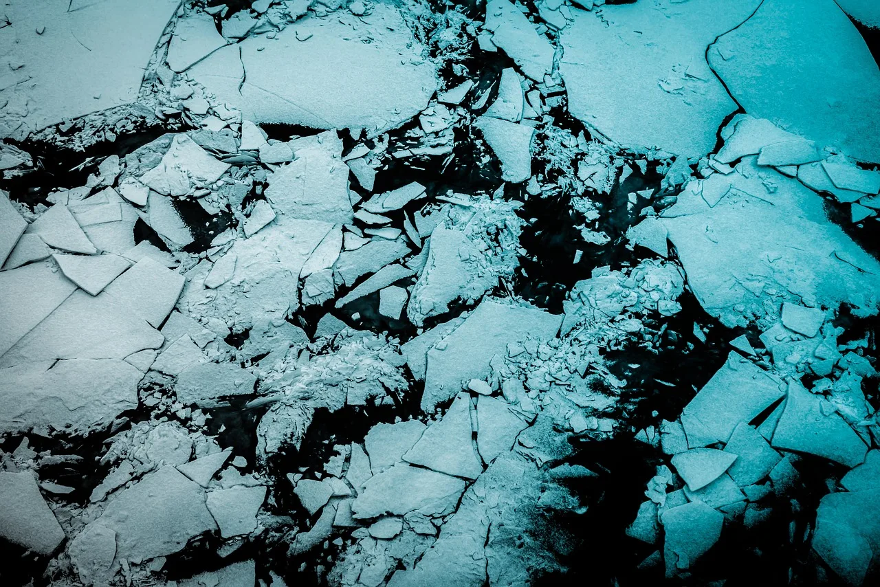
Sea ice concentration mapping is currently a manual craft. National ice services such as the Canadian Ice Service (CIS) and the U.S National Ice Center have analysts look at synthetic aperture radar (SAR) imagery, hand-draw polygons around regions of similar-looking ice, and assign each polygon a concentration value on an arbitrary scale. It works, but this opens a limitation of manual interpretation: it’s subjective, coarse, and slow to publish. In a region where shipping routes are opening up as the ice retreats, latency and resolution both matter.

Foundation models promise faster, more consistent, higher-resolution mapping without training a model from scratch on radar data. We wanted to test whether that promise holds for sea ice. Specifically: does a classifier that uses Clay’s geospatial embeddings as features predict ice concentration better than one that doesn’t? We trained three configurations to find out, one baseline built on radar statistics, weather, and land distance alone, and two that add Clay embeddings in different ways. In this first set of experiments, the embeddings didn’t improve results.

The Approach

The Arctic Sea Ice Project classifies every 320m x 320m grid in Hudson Bay into one of eleven ice concentration classes (0 = open water, 10 = fully ice-covered), directly matching the SIGRID-3 scheme ice services already use. We feed pixel chips of Sentinel-1 EW SAR imagery into Clay v1.5, a pretrained geospatial foundation model. 

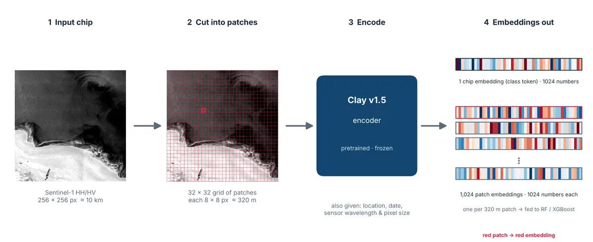
For this modelling pass, we’re using Clay as is, without fine tuning. We break each satellite radar image (scene) into thousands of patches, and then using Clay, we create thousands of embedding vectors from those patches. These vectors, along with other forms of data such as ERA5 weather data, were used in a simpler classifier that makes the actual ice-concentration predictions. 

We tested a few configurations side by side to see how much Clay embeddings actually improve our ability to predict sea ice concentration. Two configurations included Clay embeddings aggregated in different ways, and one configuration (the baseline) did not include Clay embeddings at all. By comparing the performance of these models against one another we can determine how much Clay embeddings improved the sea ice predictions. 

Training and Validation

Training was done using these three different configurations:

• Configuration 1 (baseline) — Just the basics: radar signal statistics, plus weather and land-distance data. This is the baseline everything else is compared against.
• Configuration 2 — Everything in Configuration 1, plus Clay’s AI-vision features for each small patch of the image.
• Configuration 3 — Everything in Configuration 2, plus one more Clay feature summarizing the whole image chip as a single unit.

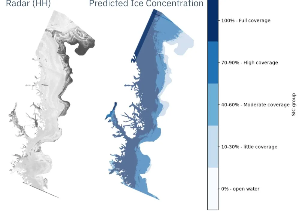
Evaluating geospatial models takes care. Patches from the same SAR scene are spatially adjacent and look alike, so scoring a model on patches from a scene it was trained on inflates results. A random split would have given us near-perfect scores that mean nothing. So, we evaluated the model against a scene it had never seen. On that stricter test, predictions landed about one ice-coverage category from the truth on average.

Once we corrected that and checked the model against a scene it had truly never seen before, the results were more honest: on average, the model’s guesses landed about one ice-coverage category off from the truth. We’ve also started grouping the results into simpler, more intuitive bands (open water, light, moderate, high, and full ice coverage) rather than eleven fine-grained levels, which solved a balancing problem we had where some levels contained very little training data, resulting in untrustworthy predictions at those levels.

Where Things Stand

So far, we’ve trained on a small slice of the available data, about 10 out of 500+ satellite scenes, as an early sanity check rather than a final effort. The results have been a genuine learning experience. We’ve found, somewhat surprisingly, that adding Clay’s AI-vision features hasn’t clearly outperformed just using the raw radar statistics yet; though, at this small scale and with an evaluation that doesn’t fully test generalization, that’s still an open question rather than a final verdict.

From here, our priority is to explore other ways we can turn Clay embeddings into features, train on much more of the available data, set aside real scenes purely for testing instead of borrowing from the training set, and run a fairer comparison to figure out whether Clay’s AI-vision features earn their cost once the model has more to learn from. The pipeline works end to end, from raw radar image to a labeled ice map, which means the next stretch of work is all about model experimenting and improvement.