STAC it up - A STAC tutorial

STAC it up – A STAC tutorial

Tomer Rockman June 21, 2022

In today’s post I will be describing the process of taking a federal Canadian dataset and creating a SpatioTemporal Asset Catalog (STAC) using python. STAC is quickly becoming the metadata standard in the open-source geospatial community and for good reason. STAC allows data providers a great way to ~~provide~~ relay standardized information about their dataset to a potential user without handing over the data itself. On the user end, it helps create workflows and pipelines that can keep data analysis completely in the cloud.

For those who have not yet encountered STAC, the website provides a great description of the function it provides:

The SpatioTemporal Asset Catalog (STAC) specification provides a common language to describe a range of geospatial information, so it can more easily be indexed and discovered. A ‘spatiotemporal asset’ is any file that represents information about the earth captured in a certain space and time.
https://stacspec.org/

STAC provides a ‘signpost’ for your dataset, giving information about what data exists within the dataset and where (in the cloud) to find it.

Getting Started

Every STAC process should begin with a look at the data. We’ll need to have at least a basic understanding of the data to make sure that the way we want to organise and divide the data makes sense.

For this tutorial we’ll be using the Canada Landsat Disturbance (CanLaD) dataset that provides information on forest disturbance in Canada between 1985-2015. The dataset relates to a recent area of research for us here at Sparkgeo, investigating the connection between fires and flooding.

Below I use the rasterio python package to plot a snippet of the ‘type’ raster looking at the Okanagan valley, an area with mixed disturbance. Forest loss to fire is shown in dark blue, harvest in yellow.

This data consists of two separate rasters. Each raster provides information on forest disturbance that took place between 1984 and 2015. The ‘type’ raster contains one band with a value of 1 representing fire and 2 representing harvest. The ‘latest year’ raster contains one band with the year that the latest disturbance occurred (1984-2015). The data is based off the 30m Landsat grid and shares its resolution.

import rasterio
from matplotlib import pyplot 

src = rasterio.open("Okanagan-Disturbance.tiff")
pyplot.figure(figsize=(15,15))
pyplot.imshow(src.read(1), cmap = 'viridis')
pyplot.show()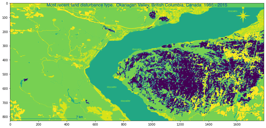

Libraries and Setup

Now that we have an understanding of the structure of our data we begin the STAC creation process by installing some essential python libraries. We use PySTAC to create and manipulate our STAC data and Rasterio for some exploratory analysis.

PySTAC

PySTAC is the most important library for working with STAC in Python 3. Some features of PySTAC:

Reading and writing STAC version 1.0.
In-memory manipulation of STAC catalogs.
Extend the I/O of STAC metadata to provide support for other platforms (e.g. cloud providers).
Easy, efficient crawling of STAC catalogs. STAC objects are only read in when needed.

PyProj

PyProj is a Python interface to PROJ (cartographic projections and coordinate transformations library). This is used for reprojecting coordinates later on in the tutorial.

We’ll also use some of the usual geospatial libraries which I import here along with some STAC extensions which I’ll talk about later.

import pystac
from urllib.request import urlopen, urlretrieve
import requests
import json
import fsspec
from typing import Any, Dict
from pyproj import CRS, Proj
from shapely.geometry import Polygon, box
from typing import Any, Dict, List, Optional
from datetime import datetime
from shapely.geometry import mapping as geojson_mapping
from pystac.extensions.file import FileExtension
from pystac import Link, Provider, ProviderRole

from pystac.extensions.projection import ProjectionExtension
from pystac.extensions.scientific import ScientificExtension
from pystac.extensions.label import (
    LabelClasses,
    LabelExtension,
    LabelTask,
    LabelType,
)

I’ll also declare this function which is a modified version of this script. This function captures data from a provided JSON-LD metadata file, which we’ll pass in later. The Canadian Federal datasets are great for providing this additional info and it makes our jobs much easier too.

def get_metadata(metadata_url: str) -> Dict[str, Any]:
    """Gets metadata from the various formats published by NRCan.
    Args:
        metadata_url (str): url to get metadata from.
    Returns:
        dict: Metadata.
    """
    if metadata_url.endswith(".jsonld"):
        if metadata_url.startswith("http"):
            metadata_response = requests.get(metadata_url)
            jsonld_response = metadata_response.json()
        else:
            with open(metadata_url) as f:
                jsonld_response = json.load(f)

        tiff_metadata = [
            i for i in jsonld_response.get("@graph")
            if i.get("dct:format") == "TIFF"
        ][0]

        geom_obj = next(
            (x["locn:geometry"] for x in jsonld_response["@graph"]
             if "locn:geometry" in x.keys()),
            [],
        )  # type: Any
        geom_metadata = next(
            (json.loads(x["@value"])
             for x in geom_obj if x["@type"].startswith("http")),
            None,
        )
        if not geom_metadata:
            raise ValueError("Unable to parse geometry metadata from jsonld")

        description_metadata = [
            i for i in jsonld_response.get("@graph")
            if "dct:description" in i.keys()
        ][0]

        metadata = {
            "tiff_metadata": tiff_metadata,
            "geom_metadata": geom_metadata,
            "description_metadata": description_metadata
        }

        return metadata
    else:
        # only jsonld support.
        raise NotImplementedError()

Creating the STAC: Items

With that housekeeping out of the way let’s move to actually create the STAC item. An item is the second smallest STAC object we can create. If a collection is like a molecule then an item is an individual atom. Each item holds information about a single file, and includes a link to that file in the form of an asset.

We’re going to add lots of information to our item including extensions used to fill out data that doesn’t fall under the native STAC spec.

First we’re going to use the metadata to get some basic properties. Let’s take a look and see what we can learn from it:

metadata_url = 'https://open.canada.ca/data/en/dataset/add1346b-f632-4eb9-a83d-a662b38655ad.jsonld'
metadata = get_metadata(metadata_url)

Let’s take a look at this metadata:

{'description_metadata': {'@id': 'https://open.canada.ca/dataset/add1346b-f632-4eb9-a83d-a662b38655ad',
  'dcat:contactPoint': {'@id': '_:N5bedf9493e5a4b20968e0716db2f331e'},
  'dcat:distribution': [{'@id': 'https://open.canada.ca/dataset/add1346b-f632-4eb9-a83d-a662b38655ad/resource/ec300cb7-e909-4ec3-8c06-7da02995abe6'},
   {'@id': 'https://open.canada.ca/dataset/add1346b-f632-4eb9-a83d-a662b38655ad/resource/c43074cd-b0f9-429c-8733-b31f13d57daa'},
   {'@id': 'https://open.canada.ca/dataset/add1346b-f632-4eb9-a83d-a662b38655ad/resource/613624c6-32c9-42f9-b53d-5da69a035288'},
   {'@id': 'https://open.canada.ca/dataset/add1346b-f632-4eb9-a83d-a662b38655ad/resource/13f1a8a7-0b4c-42b8-9ac6-69538202dfbd'},
   {'@id': 'https://open.canada.ca/dataset/add1346b-f632-4eb9-a83d-a662b38655ad/resource/717f6d31-03ea-4d39-b180-d9ac5f41c84d'},
   {'@id': 'https://open.canada.ca/dataset/add1346b-f632-4eb9-a83d-a662b38655ad/resource/964d538b-cb40-4cd0-944f-573ff0138db9'},
   {'@id': 'https://open.canada.ca/dataset/add1346b-f632-4eb9-a83d-a662b38655ad/resource/978c00bb-6b8f-41f0-9d02-7e92f75d43b0'},
   {'@id': 'https://open.canada.ca/dataset/add1346b-f632-4eb9-a83d-a662b38655ad/resource/4ff7bcb6-90dc-4529-99e3-d5cf15e4de17'}],
  'dct:accrualPeriodicity': 'as_needed',
  'dct:description': 'This data publication contains a set of files in which areas affected by fire or by harvest from 1984 to 2015 are identified at the level of individual 30m pixels on the Landsat grid. Details of the product development can be found in Guindon et al (2018).',
  'dct:identifier': 'add1346b-f632-4eb9-a83d-a662b38655ad',
  'dct:issued': {'@type': 'xsd:dateTime',
   '@value': '2018-01-10T15:25:04.409973'},
  'dct:modified': {'@type': 'xsd:dateTime',
   '@value': '2020-12-09T18:27:48.277180'},
  'dct:publisher': {'@id': 'https://open.canada.ca/organization/9391E0A2-9717-4755-B548-4499C21F917B'},
  'dct:spatial': {'@id': '_:Nc3bed52736a546a0a33280541b9cc986'},
  'dct:title': 'Canada Landsat Disturbance (CanLaD) 2017',
  'schema:itemtype': {'@id': 'dcat:Dataset'}},
 'geom_metadata': {'coordinates': [[[-141.003, 41.6755],
    [-52.6174, 41.6755],
    [-52.6174, 83.113],
    [-141.003, 83.113],
    [-141.003, 41.6755]]],
  'type': 'Polygon'},
 'tiff_metadata': {'@id': 'https://open.canada.ca/dataset/add1346b-f632-4eb9-a83d-a662b38655ad/resource/978c00bb-6b8f-41f0-9d02-7e92f75d43b0',
  'dcat:accessURL': {'@id': 'https://ftp.maps.canada.ca/pub/nrcan_rncan/Forests_Foret/landsat_disturbance/1984_2015/CanLaD_20151984_latest_type.tif'},
  'dct:format': 'TIFF',
  'dct:language': 'zxx',
  'dct:title': 'Type of the latest forest disturbance (fire=1 or harvest=2), 1984 to 2015',
  'schema:itemtype': {'@id': 'dcat:Distribution'}}}

The title, description, and date are all important parts of the item. Note that title and description are added into a dictionary called properties.

The properties dictionary holds additional metadata that falls outside of the standard STAC item args. Check out the docs here for more info.

title = metadata["tiff_metadata"]["dct:title"]
description = metadata["description_metadata"]["dct:description"]
properties = {
    "title": title,
    "description": description,
}

start_datetime = datetime.strptime('1984', "%Y")  
end_datetime = datetime.strptime('2015', "%Y")

Here I use rasterio to extract and transform some important spatial data for our STAC. STAC spec requires that geometry data be in EPSG:4326, but our projection extension requires the native geometry (so that the user can know what projection the data is in) and bounding box (bbox), so we make sure to provide both where necessary.

cog_href = 'CanLaD_20151984_latest_type.tif'


with rasterio.open(cog_href) as dataset:
  cog_bbox = list(dataset.bounds)
  cog_transform = list(dataset.transform)
  cog_shape = [dataset.height, dataset.width]

  transformer = Proj.from_crs(CRS.from_epsg(DATA_EPSG),
                              CRS.from_epsg(4326),
                              always_xy=True)
  bbox = list(
      transformer.transform_bounds(dataset.bounds.left,
                                    dataset.bounds.bottom,
                                    dataset.bounds.right,
                                    dataset.bounds.top))
  geometry = geojson_mapping(box(*bbox, ccw=True))

Now we’ll declare and initialize our item using the information we’ve collected so far. We pass in a unique id, our geometry and bounding box, start and end date times, the properties dictionary, and an empty list of STAC extensions.

This item is made for the raster related to most recent disturbance type, so we’ll call it type_raster. The last list, stac_extensions, will be filled using the applicable extensions later in this tutorial.

# Create item
item = pystac.Item(
  id='type_raster',
  geometry=geometry,
  bbox=bbox,
  datetime=start_datetime,
  properties=properties,
  stac_extensions=[],
)

item.common_metadata.start_datetime = start_datetime
item.common_metadata.end_datetime = end_datetime

Assets

An asset is an object that contains a URI to the data associated with an item. In our case, we will be adding two assets to each item in our collection. One asset is for the data itself while the other is for its metadata.

Assets can either be created inside the add_asset <make sure you're being consistent in highlighting functions and fields from your code using the inline code font style. I see some cases where you do it and others where you don't function or created, then added after. You can see both methods here.

item.add_asset(
  "metadata",
  pystac.Asset(
      href=metadata_url,
      media_type=pystac.MediaType.JSON,
      roles=["metadata"],
      title="Landsat Disturbance Metadata",
  ),
)
cog_asset = pystac.Asset(
  href= cog_href,
  media_type=pystac.MediaType.COG,
  roles=[
    "data",
    "labels",
    "labels-raster",
  ],
  title="Canada Landsat Disturbance COG",
)
item.add_asset('COG', cog_asset)

Extensions

The STAC spec itself is fairly minimal, but due to its extensibility, it can become much more comprehensive. STAC extensions allow us to add tons of different data that is associated with our dataset.

Extensions are JSON fields that are associated with either items, assets, collection, or catalogs. In most cases when you are creating a STAC you will need to dig into extensions in order to properly describe your data.

Check out the extensions overview page to see what extensions might be useful for your data. One can add as many extensions as is applicable. For the purposes of this workshop we’ll be focussing on item and asset extensions.

Projection Extension

We’ll start with the projection extension which provides a way to describe Items whose assets are in a geospatial projection. More info about this extension can be found here.

item_projection = ProjectionExtension.ext(item, add_if_missing=True)

item_projection.epsg = DATA_EPSG
item_projection.wkt2 = DATA_CRS_WKT
item_projection.bbox = cog_bbox
item_projection.transform = cog_transform
item_projection.shape = cog_shape

Scientific Extension

The scientific extension is used when an item contains data linked to a scientific publication, it tells a user which publication it originates from and how to cite it. I grabbed the DOI and the citation from here. To learn more about the scientific extensions you can read the docs here.

CITATION = 'Guindon, L.; Bernier, P.Y.; Gauthier, S.; Stinson, G.; Villemaire, P.; Beaudoin, A. 2018. Missing forest cover gains in boreal forests explained. Ecosphere, 9 (1) Article e02094.'
DOI = '10.1002/ecs2.2094'

item_sci = ScientificExtension.ext(item, add_if_missing=True)
item_sci.doi = DOI
item_sci.citation = CITATION

Label Extension

Though intended to support labeled AOIs with ML models the label extension is useful for any data that contains labeled AOIs. We use it here to provide info on the the classes in our raster data. More info on the label extension can be found here.

CLASSIFICATION_VALUES = {1: 'fire',
                         2: 'harvest'}

item_label = LabelExtension.ext(item, add_if_missing=True)
item_label.label_type = LabelType.RASTER
item_label.label_tasks = [LabelTask.CLASSIFICATION]
item_label.label_properties = None
item_label.label_description = "Fire or Harvest"
item_label.label_classes = [LabelClasses.create(list(CLASSIFICATION_VALUES.values()), None)]

File Extension

Provides basic info such as size, data type and checksum for assets in an item or collection. The file extension can also be used to map our classification values. More info on the file extension can be found here.

from pystac.extensions.file import MappingObject

cog_asset_file = FileExtension.ext(cog_asset, add_if_missing=True)

mapping = [
  MappingObject.create(values=[value], summary=summary)
  for value, summary in CLASSIFICATION_VALUES.items()
]
cog_asset_file.values = mapping

with fsspec.open(cog_href) as file:
  size = file.size
  cog_asset_file.size = size

Let’s take a look at what our item currently looks like:

{'assets': {'COG': {'file:size': 290194588,
   'file:values': [{'summary': 'fire', 'values': [1]},
    {'summary': 'harvest', 'values': [2]}],
   'href': 'CanLaD_20151984_latest_type.tif',
   'roles': ['data', 'labels', 'labels-raster'],
   'title': 'Canada Landsat Disturbance COG',
   'type': <MediaType.COG: 'image/tiff; application=geotiff; profile=cloud-optimized'>},
  'metadata': {'href': 'https://open.canada.ca/data/en/dataset/add1346b-f632-4eb9-a83d-a662b38655ad.jsonld',
   'roles': ['metadata'],
   'title': 'Landsat Disturbance Metadata',
   'type': <MediaType.JSON: 'application/json'>}},
 'bbox': [29.208147682613188,
  40.20704372347072,
  134.7641106438931,
  80.41031119985433],
 'geometry': {'coordinates': (((134.7641106438931, 40.20704372347072),
    (134.7641106438931, 80.41031119985433),
    (29.208147682613188, 80.41031119985433),
    (29.208147682613188, 40.20704372347072),
    (134.7641106438931, 40.20704372347072)),),
  'type': 'Polygon'},
 'id': 'type_raster',
 'links': [{'href': 'https://doi.org/10.1002/ecs2.2094',
   'rel': <ScientificRelType.CITE_AS: 'cite-as'>}],
 'properties': {'datetime': '1984-01-01T00:00:00Z',
  'description': 'This data publication contains a set of files in which areas affected by fire or by harvest from 1984 to 2015 are identified at the level of individual 30m pixels on the Landsat grid. Details of the product development can be found in Guindon et al (2018).',
  'end_datetime': '2015-01-01T00:00:00Z',
  'label:classes': [{'classes': ['fire', 'harvest'], 'name': None}],
  'label:description': 'Fire or Harvest',
  'label:properties': None,
  'label:tasks': [<LabelTask.CLASSIFICATION: 'classification'>],
  'label:type': <LabelType.RASTER: 'raster'>,
  'proj:bbox': [-2341500.0, 5863500.0, 3010500.0, 9436500.0],
  'proj:epsg': 3979,
  'proj:shape': [119100, 178400],
  'proj:transform': [30.0,
   0.0,
   -2341500.0,
   0.0,
   -30.0,
   9436500.0,
   0.0,
   0.0,
   1.0],
  'proj:wkt2': 'PROJCRS["NAD83(CSRS) / Canada Atlas Lambert",BASEGEOGCRS["NAD83(CSRS)",DATUM["NAD83 Canadian Spatial Reference System",ELLIPSOID["GRS 1980",6378137,298.257222101,LENGTHUNIT["metre",1]]],PRIMEM["Greenwich",0,ANGLEUNIT["degree",0.0174532925199433]],ID["EPSG",4617]],CONVERSION["Canada Atlas Lambert",METHOD["Lambert Conic Conformal (2SP)",ID["EPSG",9802]],PARAMETER["Latitude of false origin",49,ANGLEUNIT["degree",0.0174532925199433],ID["EPSG",8821]],PARAMETER["Longitude of false origin",-95,ANGLEUNIT["degree",0.0174532925199433],ID["EPSG",8822]],PARAMETER["Latitude of 1st standard parallel",49,ANGLEUNIT["degree",0.0174532925199433],ID["EPSG",8823]],PARAMETER["Latitude of 2nd standard parallel",77,ANGLEUNIT["degree",0.0174532925199433],ID["EPSG",8824]],PARAMETER["Easting at false origin",0,LENGTHUNIT["metre",1],ID["EPSG",8826]],PARAMETER["Northing at false origin",0,LENGTHUNIT["metre",1],ID["EPSG",8827]]],CS[Cartesian,2],AXIS["(E)",east,ORDER[1],LENGTHUNIT["metre",1]],AXIS["(N)",north,ORDER[2],LENGTHUNIT["metre",1]],USAGE[SCOPE["Transformation of coordinates at 5m level of accuracy."],AREA["Canada - onshore and offshore - Alberta; British Columbia; Manitoba; New Brunswick; Newfoundland and Labrador; Northwest Territories; Nova Scotia; Nunavut; Ontario; Prince Edward Island; Quebec; Saskatchewan; Yukon."],BBOX[38.21,-141.01,86.46,-40.73]],ID["EPSG",3979]]',
  'sci:citation': 'Guindon, L.; Bernier, P.Y.; Gauthier, S.; Stinson, G.; Villemaire, P.; Beaudoin, A. 2018. Missing forest cover gains in boreal forests explained. Ecosphere, 9 (1) Article e02094.',
  'sci:doi': '10.1002/ecs2.2094',
  'start_datetime': '1984-01-01T00:00:00Z',
  'title': 'Type of the latest forest disturbance (fire=1 or harvest=2), 1984 to 2015'},
 'stac_extensions': ['https://stac-extensions.github.io/projection/v1.0.0/schema.json',
  'https://stac-extensions.github.io/scientific/v1.0.0/schema.json',
  'https://stac-extensions.github.io/label/v1.0.1/schema.json',
  'https://stac-extensions.github.io/file/v2.0.0/schema.json'],
 'stac_version': '1.0.0',
 'type': 'Feature'}

Collection Creation

Next we’re going to create a collection. A collection contains fields that describe a group of items that share properties and metadata. In our example our collection will hold the ‘type’ and ‘latest year’ raster data sets.

title = metadata["tiff_metadata"]["dct:title"]
description = metadata["description_metadata"]["dct:description"]

license = "OGL-Canada-2.0"
license_link = Link(
  rel="license",
  target="https://open.canada.ca/en/open-government-licence-canada",
  title="Open Government Licence - Canada",
)

start_datetime = datetime.strptime('1984', "%Y")  
end_datetime = datetime.strptime('2015', "%Y")


CANLAD_PROVIDER = Provider(
    name="Open Government",
    roles=[
        ProviderRole.HOST,
        ProviderRole.LICENSOR,
        ProviderRole.PROCESSOR,
        ProviderRole.PRODUCER,
    ],
    url=
    "https://open.canada.ca/data/en/dataset/add1346b-f632-4eb9-a83d-a662b38655ad"
)


collection = pystac.Collection(
  id='CanLaD',
  title=title,
  description=description,
  providers=[CANLAD_PROVIDER],
  license=license,
  extent=pystac.Extent(
    pystac.SpatialExtent([bbox]),
    pystac.TemporalExtent([[start_datetime, end_datetime]]),
  ),
  catalog_type=pystac.CatalogType.RELATIVE_PUBLISHED,
)
collection.add_link(license_link)

Collection Assets

Just like items, collection can also have assets. Here we add the metadata as an asset.

collection.add_asset(
  "metadata",
  pystac.Asset(
    href=metadata_url,
    media_type=pystac.MediaType.JSON,
    roles=["metadata"],
    title="Canada Landsat Disturbance metadata",
  )
)

Collection Extensions

Collections can also have extensions, some of these are already familiar. Here we add the scientific, label and projection extensions just like we did before:

collection_label = LabelExtension.summaries(collection,
                                            add_if_missing=True)
collection_label.label_type = [LabelType.RASTER]
collection_label.label_tasks = [LabelTask.CLASSIFICATION]
collection_label.label_properties = None
collection_label.label_classes = [
    LabelClasses.create(list(CLASSIFICATION_VALUES.values()), None)
]

collection_proj = ProjectionExtension.summaries(collection,
                                                add_if_missing=True)
collection_proj.epsg = [DATA_EPSG]

collection_sci = ScientificExtension.ext(collection, add_if_missing=True)
collection_sci.doi = DOI
collection_sci.citation = CITATION

STACification

Finally we’re ready to assemble our STAC. This is fairly simple and just involves setting the items self_href which makes sure that there is a link in the item to itself. We then do the same for the collection. Lastly we add the item to the collection:

item.set_self_href('item.json')
collection.set_self_href('collection.json')
collection.add_item(item)

Now lets have a look at our STAC. The collection looks like this:

{'assets': {'metadata': {'href': 'https://open.canada.ca/data/en/dataset/add1346b-f632-4eb9-a83d-a662b38655ad.jsonld',
   'roles': ['metadata'],
   'title': 'Canada Landsat Disturbance metadata',
   'type': <MediaType.JSON: 'application/json'>}},
 'description': 'This data publication contains a set of files in which areas affected by fire or by harvest from 1984 to 2015 are identified at the level of individual 30m pixels on the Landsat grid. Details of the product development can be found in Guindon et al (2018).',
 'extent': {'spatial': {'bbox': [[29.208147682613188,
     40.20704372347072,
     134.7641106438931,
     80.41031119985433]]},
  'temporal': {'interval': [['1984-01-01T00:00:00Z',
     '2015-01-01T00:00:00Z']]}},
 'id': 'CanLaD',
 'license': 'OGL-Canada-2.0',
 'links': [{'href': './collection.json',
   'rel': <RelType.ROOT: 'root'>,
   'title': 'Type of the latest forest disturbance (fire=1 or harvest=2), 1984 to 2015',
   'type': <MediaType.JSON: 'application/json'>},
  {'href': 'https://open.canada.ca/en/open-government-licence-canada',
   'rel': 'license',
   'title': 'Open Government Licence - Canada'},
  {'href': 'https://doi.org/10.1002/ecs2.2094',
   'rel': <ScientificRelType.CITE_AS: 'cite-as'>},
  {'href': '/content/collection.json',
   'rel': <RelType.SELF: 'self'>,
   'type': <MediaType.JSON: 'application/json'>},
  {'href': './type_raster/type_raster.json',
   'rel': <RelType.ITEM: 'item'>,
   'type': <MediaType.JSON: 'application/json'>}],
 'providers': [{'name': 'Open Government',
   'roles': [<ProviderRole.HOST: 'host'>,
    <ProviderRole.LICENSOR: 'licensor'>,
    <ProviderRole.PROCESSOR: 'processor'>,
    <ProviderRole.PRODUCER: 'producer'>],
   'url': 'https://open.canada.ca/data/en/dataset/add1346b-f632-4eb9-a83d-a662b38655ad'}],
 'sci:citation': 'Guindon, L.; Bernier, P.Y.; Gauthier, S.; Stinson, G.; Villemaire, P.; Beaudoin, A. 2018. Missing forest cover gains in boreal forests explained. Ecosphere, 9 (1) Article e02094.',
 'sci:doi': '10.1002/ecs2.2094',
 'stac_extensions': ['https://stac-extensions.github.io/label/v1.0.1/schema.json',
  'https://stac-extensions.github.io/projection/v1.0.0/schema.json',
  'https://stac-extensions.github.io/scientific/v1.0.0/schema.json'],
 'stac_version': '1.0.0',
 'summaries': {'label:classes': [{'classes': ['fire', 'harvest'],
    'name': None}],
  'label:tasks': [<LabelTask.CLASSIFICATION: 'classification'>],
  'label:type': [<LabelType.RASTER: 'raster'>],
  'proj:epsg': [3979]},
 'title': 'Type of the latest forest disturbance (fire=1 or harvest=2), 1984 to 2015',
 'type': 'Collection'}

Note the self link as well as the link to the item we added. Speaking of our item lets take a look at that:

{'assets': {'COG': {'file:size': 604432423,
   'file:values': [{'summary': 'fire', 'values': [1]},
    {'summary': 'harvest', 'values': [2]}],
   'href': '../CanLaD_20151984_latest_YRT2.tif',
   'roles': ['data', 'labels', 'labels-raster'],
   'title': 'Canada Landsat Disturbance COG',
   'type': <MediaType.COG: 'image/tiff; application=geotiff; profile=cloud-optimized'>},
  'metadata': {'href': 'https://open.canada.ca/data/en/dataset/add1346b-f632-4eb9-a83d-a662b38655ad.jsonld',
   'roles': ['metadata'],
   'title': 'Landsat Disturbance Metadata',
   'type': <MediaType.JSON: 'application/json'>}},
 'bbox': [29.208147682613188,
  40.20704372347072,
  134.7641106438931,
  80.41031119985433],
 'collection': 'CanLaD',
 'geometry': {'coordinates': (((134.7641106438931, 40.20704372347072),
    (134.7641106438931, 80.41031119985433),
    (29.208147682613188, 80.41031119985433),
    (29.208147682613188, 40.20704372347072),
    (134.7641106438931, 40.20704372347072)),),
  'type': 'Polygon'},
 'id': 'type_raster',
 'links': [{'href': 'https://doi.org/10.1002/ecs2.2094',
   'rel': <ScientificRelType.CITE_AS: 'cite-as'>},
  {'href': '../collection.json',
   'rel': <RelType.ROOT: 'root'>,
   'title': 'Type of the latest forest disturbance (fire=1 or harvest=2), 1984 to 2015',
   'type': <MediaType.JSON: 'application/json'>},
  {'href': '../collection.json',
   'rel': <RelType.PARENT: 'parent'>,
   'title': 'Type of the latest forest disturbance (fire=1 or harvest=2), 1984 to 2015',
   'type': <MediaType.JSON: 'application/json'>},
  {'href': '/content/type_raster/type_raster.json',
   'rel': <RelType.SELF: 'self'>,
   'type': <MediaType.JSON: 'application/json'>},
  {'href': '../collection.json',
   'rel': <RelType.COLLECTION: 'collection'>,
   'title': 'Type of the latest forest disturbance (fire=1 or harvest=2), 1984 to 2015',
   'type': <MediaType.JSON: 'application/json'>}],
 'properties': {'datetime': '1984-01-01T00:00:00Z',
  'description': 'This data publication contains a set of files in which areas affected by fire or by harvest from 1984 to 2015 are identified at the level of individual 30m pixels on the Landsat grid. Details of the product development can be found in Guindon et al (2018).',
  'end_datetime': '2015-01-01T00:00:00Z',
  'label:classes': [{'classes': ['fire', 'harvest'], 'name': None}],
  'label:description': 'Fire or Harvest',
  'label:properties': None,
  'label:tasks': [<LabelTask.CLASSIFICATION: 'classification'>],
  'label:type': <LabelType.RASTER: 'raster'>,
  'proj:bbox': [-2341500.0, 5863500.0, 3010500.0, 9436500.0],
  'proj:epsg': 3979,
  'proj:shape': [119100, 178400],
  'proj:transform': [30.0,
   0.0,
   -2341500.0,
   0.0,
   -30.0,
   9436500.0,
   0.0,
   0.0,
   1.0],
  'proj:wkt2': 'PROJCRS["NAD83(CSRS) / Canada Atlas Lambert",BASEGEOGCRS["NAD83(CSRS)",DATUM["NAD83 Canadian Spatial Reference System",ELLIPSOID["GRS 1980",6378137,298.257222101,LENGTHUNIT["metre",1]]],PRIMEM["Greenwich",0,ANGLEUNIT["degree",0.0174532925199433]],ID["EPSG",4617]],CONVERSION["Canada Atlas Lambert",METHOD["Lambert Conic Conformal (2SP)",ID["EPSG",9802]],PARAMETER["Latitude of false origin",49,ANGLEUNIT["degree",0.0174532925199433],ID["EPSG",8821]],PARAMETER["Longitude of false origin",-95,ANGLEUNIT["degree",0.0174532925199433],ID["EPSG",8822]],PARAMETER["Latitude of 1st standard parallel",49,ANGLEUNIT["degree",0.0174532925199433],ID["EPSG",8823]],PARAMETER["Latitude of 2nd standard parallel",77,ANGLEUNIT["degree",0.0174532925199433],ID["EPSG",8824]],PARAMETER["Easting at false origin",0,LENGTHUNIT["metre",1],ID["EPSG",8826]],PARAMETER["Northing at false origin",0,LENGTHUNIT["metre",1],ID["EPSG",8827]]],CS[Cartesian,2],AXIS["(E)",east,ORDER[1],LENGTHUNIT["metre",1]],AXIS["(N)",north,ORDER[2],LENGTHUNIT["metre",1]],USAGE[SCOPE["Transformation of coordinates at 5m level of accuracy."],AREA["Canada - onshore and offshore - Alberta; British Columbia; Manitoba; New Brunswick; Newfoundland and Labrador; Northwest Territories; Nova Scotia; Nunavut; Ontario; Prince Edward Island; Quebec; Saskatchewan; Yukon."],BBOX[38.21,-141.01,86.46,-40.73]],ID["EPSG",3979]]',
  'sci:citation': 'Guindon, L.; Bernier, P.Y.; Gauthier, S.; Stinson, G.; Villemaire, P.; Beaudoin, A. 2018. Missing forest cover gains in boreal forests explained. Ecosphere, 9 (1) Article e02094.',
  'sci:doi': '10.1002/ecs2.2094',
  'start_datetime': '1984-01-01T00:00:00Z',
  'title': 'Type of the latest forest disturbance (fire=1 or harvest=2), 1984 to 2015'},
 'stac_extensions': ['https://stac-extensions.github.io/projection/v1.0.0/schema.json',
  'https://stac-extensions.github.io/scientific/v1.0.0/schema.json',
  'https://stac-extensions.github.io/label/v1.0.1/schema.json',
  'https://stac-extensions.github.io/file/v2.0.0/schema.json'],
 'stac_version': '1.0.0',
 'type': 'Feature'}

We can see that the item now contains a self link as well as a link to our collection!

The last thing to do is validate and save our objects. Validation ensures that our STAC objects are properly formed and checks for things like incomplete fields or incorrect syntax. PyStac performs validation and saving, in two easy steps:

item.validate()
collection.validate()

item.save_object()
collection.save_object()

And that’s it! Congrats you’ve officially created a STAC for this dataset! Now go check out the notebook here and see if you can create an item for the other raster and add it to our collection.