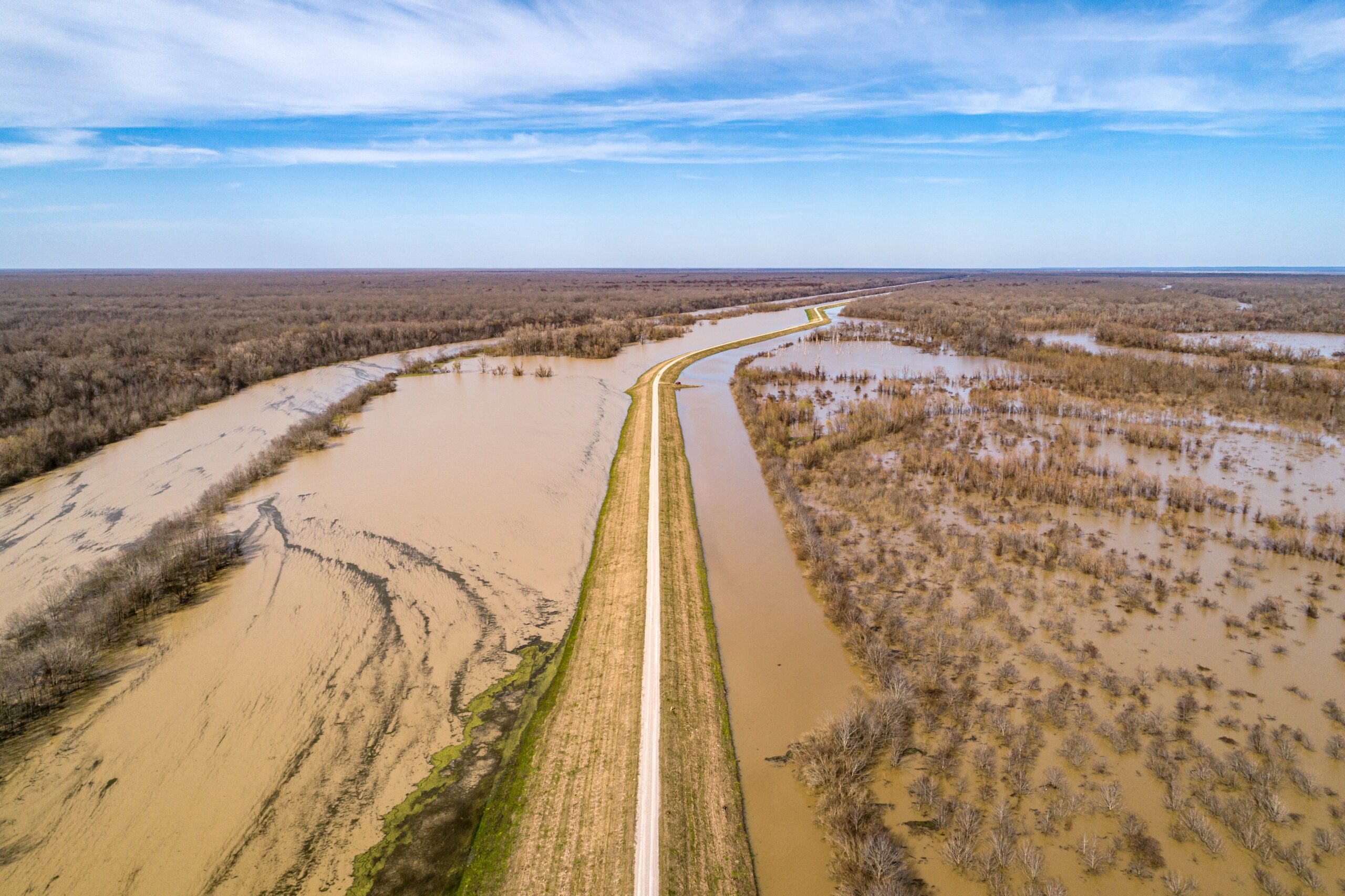
The recent flooding in British Columbia is a harsh reminder that climate change is not a hypothetical scenario that lies somewhere in the future; its effects are being felt right now. Unfortunately, events like these floods and the devastating heat dome this summer are likely to become more common and more pronounced in the future. 

To reduce the economic and human losses from severe weather events we must ensure that our infrastructure is capable of withstanding them. We at Sparkgeo believe that geospatial data and analysis provide critical information to help achieve this goal.

In a previous blog post we mapped the flooding of the Sumas Prairie near the city of Abbotsford using synthetic aperture radar (SAR) data. There, we highlighted how geospatial data can help to monitor and map flooding in near-real time. In this post, we go beyond simply mapping where flooding occurred to see if we can help explain the flooding.

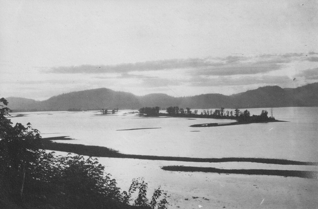
While climate change is part of the story, the flooding of Sumas Prairie is also a story of geography, and of human intervention in the landscape. The Sumas Prairie was once Sumas Lake.

Formed as the glaciers of the last ice age retreated, the lake was important for transportation and as a food source for the Semá:th first nations people that live in the region.

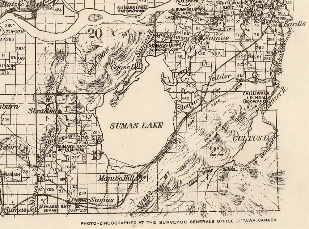
The lake was an annoyance for farmers, however, and in the 1920s it was drained, providing access to the fertile soils beneath and transforming it into one of the most productive agricultural regions in BC.

To keep it from turning back into a lake, the Sumas Prairie is managed through dikes and canals and the Barrowtown pump station. The station pumps water from the prairie uphill into the Sumas River which then drains into the Fraser River.

This system has kept the prairie dry for the last 100 years, but the lake’s return is an ever-present threat.

The cause of this most recent flooding is thought to originate not from Canada, but from across the border. The Nooksack River in northern Washington overtopped its banks on November 14th, and the floodwaters flowed north into the Sumas Prairie.

Our SAR flood map confirmed this, with a clear flood path from the Nooksack into the prairie. The Nooksack river was also the main cause of the 1990 flood, the last major flood in the region.

Topographic Analysis

To better understand this event, we need to examine the topography of the region. Luckily, high resolution Lidar elevation data was available over both Abbotsford and northern Washington. This allowed us to get a detailed picture of the landscape.

The animation below shows a true colour satellite image of the area, followed by a lidar digital elevation model (DEM). Elevation values in the DEM are symbolized using a colour gradient with low values shown as dark purple and high values shown as bright white.

In the 2nd frame of the animation, the colour gradient ranges from 0 to 200 meters above sea level. Here we see that both the Sumas Prairie and the Nooksack river lie at a very low elevation.

The prairie itself is bounded by mountains to the north and south. This condition may have contributed to the flooding, with rain running off the mountains into the valley below.

But this colour scale is too wide to tell the full story. In the 3rd frame, we increase the contrast of the image by compressing the colour scale between 0 and 30 meters. This reduces detail for higher elevations, but allows more information to be discriminated at lower elevations. 

With this narrower colour scale we can see that the Nooksack river essentially runs into a fork in the road around the town of Everson. This is shown in the animation below.

From here the river runs West toward the town of Lynden before eventually discharging into the Pacific Ocean; however, water outside the confines of the stream channel seems equally likely to run north-east instead of west, straight into the low lying Sumas Prairie.

The 3rd animation frame overlays the flooding for November 16th. We see a trail of flooding shown from Everson to the Sumas Prairie, which seems to confirm the Nooksack River as the main source of this flood.

The Topographic Wetness Index

An informative metric computed from the DEM is the Topographic Wetness Index (TWI). The TWI models where water is likely to accumulate based on elevation differences across a landscape.

Essentially, the TWI indicates areas that are more likely to be wet, and can also show the most likely pathways of flowing water. The subsequent animations depict the TWI along with the DEM to help explain the flooding we saw.

The below animation shows the area of flooding between the Nooksack River and the Sumas Prairie again. The DEM is on the left and the TWI is on the right. Flooding from November 16th is overlaid on both maps.

The TWI is shown on a colour ramp from white to dark green, where darker shades indicate higher TWI (areas more likely to accumulate moisture). It should be noted that areas shown in white should not necessarily be considered dry; merely less likely to accumulate moisture.

Looking at the animation, there is a good level of agreement between areas with high TWI values and flooding.

The next animation shows the floodplain between the City of Abbotsford and the Fraser River. Unlike the Sumas Prairie, this flooding was not associated with the Nooksack river; instead, it likely came from rain flowing down from Sumas Mountain in the east and the city itself in the south.

In this animation, the DEM is colourized over a narrow range of values between 0 and 6 meters. Shown in this way, topographic sinks and barriers in the landscape become clearly visible. These features align well with areas of pooling flood water.

There is once again high correlation between high TWI and flooding. The TWI map also shows pathways for water draining from the surrounding areas into the plain. These seem to support the idea that this flooding came from the surrounding land rather than from the Fraser River.

Failing Dikes and a Lake Revived

Overwhelmed by the flooding, the Sumas dike failed in two locations on November 16th. These failures allowed floodwaters to inundate the lowest lying portions of the Sumas Prairie which were previously protected.

The animation below shows a map from the City of Abbotsford depicting the dike failure locations. These locations were digitized and overlaid on the DEM (now colourized between 0 and 10 meters), as shown in the 3rd animation frame.

In the next animation we overlay the flooding detected on November 16th and 20th.

On the 16th we can see the flooding appears to already be entering the lower lying central prairie through the failing sections of the dike, though the bulk of the water still lies south of Abbotsford, held back by the dike. By November 20th we see the dike failures have allowed the flooding to flow downhill, inundating the central prairie.

The topographic data can potentially shed some light on why these failures occurred where they did. The two animations below show zoomed-in views of the two dike failures. Both show the DEM and TWI, as well as the flooding on November 16th.

In the first animation, showing the south-west failure location, there are notably high TWI values right around the failed section. It is possible that this area accumulated a significant amount of floodwater, increasing the chances of failure at this location.

It is also worth mentioning that the failure occurred right where a road crossed over the dike, which may have been a contributing factor.

The second animation shows the north-eastern dike failure; here too we see high TWI values near the section which failed.

On the north side of the dike, the Sumas river runs parallel, with a small riparian lake just north of it. On the south side of the dike, we can see the Trans-Canada Highway at a raised elevation, itself acting as a smaller dike.

Based on this evidence it seems possible that significant amounts of water may have accumulated on both sides of the dike, weakening it and contributing to the failure here.

In the final animation below, we colourized the DEM between 0 and 3 meters. The elevation at the bottom of the Sumas Dike near the north-east section that failed was approximately 3 meters.

Depicted in this way, the DEM correlates very well with the flooding on the 20th. It also appears flooding on the 16th started at the lowest part of the prairie, the bottom of the Sumas lakebed. The DEM roughly resembles the outline of Sumas Lake as shown in the historical map up above.

The TWI by comparison with the DEM does not provide the same correlation with flooded areas. As previously mentioned, some areas shown in white may still accumulate significant moisture, especially during such a catastrophic flood event.

The TWI was also designed to characterize hydrological conditions in natural watersheds; the Sumas Prairie being an artificial area maintained through active human intervention may weaken the explanatory power of this index.

The situation in the Sumas Prairie is still ongoing. It may be weeks before some residents can return to their homes, and the cleanup will take much longer. The cost of this flood will take time to tally, but will likely be in the hundreds of millions of dollars.

A full analysis of this event is more than can be covered in a blog post; however, it is clear that there is a wealth of information conveyed by the topographic data which can aid our understanding of how this event occurred.

This same data could be used to model flooding conditions under different scenarios to understand which areas are most at risk of flooding, which portions of the dike should be reinforced, how additional dikes, natural barriers, or water diversions might mitigate a future flood, and so on. In this way, we can use geospatial data to help reduce the chances of such an event occurring again. 

Many of the harsh realities of a changing climate are now unavoidable. But by leveraging modern data practices and intelligence, and by making policy decisions that prioritize adaptation strategies, we may yet be able to avoid some of the worst consequences.

Thanks to Devin Cairns for his work on the Topographic Wetness Index used in this post. Thanks also to Chloe Papalazarou, Natalia Domarad, and James Banting for their input.